Flows

An overview of the generative artwork project titled “Flows”, by ryley-o.eth

Release Details

“Flows” is my upcoming release on Art Blocks.

Edition Size: 100
Release Date: Tuesday, June 13
Project page: http://artblocks.io/project/435

---

Displaying Flows Tokens

I made a simple tool that can help token holders download videos of their Flows tokens. It it slow and basic, and please reach out on discord or twitter if you are a token holder who would like me to render any tokens for you!
The tool is hosted on github pages here: https://ryley-o.github.io/flows-capture/

---

Overview

ryley-o.eth has a MS in Aeronautics and Astronautics, and designed commercial aircraft at Boeing before joining Art Blocks in 2021.

Flows uses the mathematics of aerodynamics to animate colorful particles and forms that move through underlying flow fields. Potential Flow Theory, a cornerstone of traditional aerodynamic analysis, is the basis for all outputs in this project.

From an engineer’s perspective, these functions are powerful tools to simulate airflow on the wing of an airplane or weather patterns over a geographical area, but rarely are we given the freedom to explore the potential for beauty. Generative art is a wonderful platform to showcase this because it is simply math and physics given shape and color.

Subtle nods to my background in the aerospace industry are given throughout the project. Outputs include particles that traverse along pathlines, simulating particle tracer analysis methods. Some palettes limit their colors to the conventional analytical color spectrum of red to blue. Regions of smooth color gradients are broken up by discontinuities, inspired by Schlieren photographs of shockwaves.

Flows, however, intentionally breaks away from many analytical conventions. This is largely representative of my personal journey out of the aerospace industry and into the world of generative art. Streamlines are replaced by winding, spiraling forms that twist through underlying scalar potential fields instead of aligning with them. Pixelated, analytical graphs are replaced with smooth GPU animations rendered in real-time.

An extra personal touch is given to this project, inspired by my son born with Down syndrome. 25% of sales above resting price and the first $10k USD of artist royalties will be donated to Zoe’s Toolbox, a charity that provides developmental assistance to children with Trisomy 21 (Down syndrome). Additionally, Token #321 will have a unique blue and yellow palette titled “Inclusion”. 100% of artist royalties from sales of that token will be donated to Down syndrome related charities, in perpetuity.

Potential Flow Theory

Potential Flow Theory is a fluid dynamics model that assumes a flow is inviscid, incompressible, and irrotational. Even though it was developed in the sixteenth century, the theory is still used by aerodynamicists today to quickly calculate the lift and moment characteristics of airfoils. Interestingly, the theory does not predict drag or stall characteristics due to viscosity being neglected, which is known as D’Alambert’s Paradox.

For those interested in the derivations of potential flow theory, a really great resource is this page: https://potentialflow.com/derivations. Note that the site also has a potential flow simulator where you can build your own flow fields!

Flows uses potential flow theory for a few reasons. The theory is simple enough that a custom implementation could be coded and stored on the blockchain. Additionally, the simplifying assumptions were appropriate for the types of flows that I wanted to depict in the project. I wanted to use a fluid dynamics model that would be able to capture the “essense” of a wingtip vortex, the like the one shown in the picture below, and potential flow theory was capable of that.

Lastly, potential flow theory has some mathematical properties that work well with computer graphics technology. When building a two-dimensional flow field, potential flow theory has two analytical scalar potential fields: the Lagrange stream function and the velocity potential, introduced by Joseph-Louis Lagrange in 1781 and 1788, respectively. Importantly, due to the mathematics of scalar potentials, the scalar values of the Lagrange stream function and velocity potential depend only on location coordinates, not upon any paths taken or surrounding flow values. This important characteristic allows the field values to be calculated at any point in a non-iterative manner. No iteration means calculations may be performed in parallel, making it possible to generate animated, high-resolution, mathematically accurate outputs with the use of shaders.

Shaders

Shaders are used in computer graphics to efficiently display complex renderings to a screen. They are generally coded for (and run on) a graphics processing unit (GPU). Shaders typically describe the traits of a vertex or pixel. Flows implements a pixel shader (sometimes called a “fragment” shader) to parallelize the potential flow calculations for each pixel of a display.

As discussed in the previous section, the values of Potential Flow Theory’s stream function and velocity potential only depend on location. Because the inputs to a pixel shader are simply the pixel coordinates on a screen, a pixel shader provides a great way to parallelize the calculation of the scalar potential values.

Flows determines a pixel’s output based on the values of the Lagrange stream function and/or the velocity potential. Using a GPU shader results in very fast performance, enabling Flows to generate animated pixel-perfect renderings of flow fields at 60 frames per second.

Building Flows

Starting with the basics of Potential flow theory and shaders, let’s take a look at how Flows generates its outputs.

Streamlines

Since streamlines are defined as paths with constant Lagrange stream function values, let’s examine an output where pixels are black, except when the cosine of the stream function value is greater 0.98, the output is white. Note that we use cosine since it is a periodic function, which will give us many streamlines across the field in regular intervals.

// pseudo-code in fragment shader
// psi is stream function value
i = cos(psi);
pixelColor = vec3(0.0);
if (i > 0.98) {
    pixelColor = vec3(1.0);
}

A sample output rendering for a randomly generated flow field with four point elements that each have vorticity and source/sink values is shown below.

Velocity Potential & Stream Function Grid

Potential Flow theory gives us two scalar values, so let’s examine the outputs of the streamlines as well as lines of constant velocity potential. As expected, the lines of velocity potential are perpendicular to the streamlines of the flow. The flow elements create a warped grid that is the true structure of a potential flow field.

// pseudo-code in fragment shader
i = cos(psi); // psi = stream function
j = cos(phi); // phi = velocity potential
flowFieldColor = vec3(0.0);
if (i > 0.98) {
    // streamline = white
    flowFieldColor = vec3(1.0);
}
if (j > 0.98) {
    // constant velocity potential = grey
    flowFieldColor = vec3(0.5);
}

Adding Color

Instead of using lines of constant color, what if we depict our flow field with colors that depend on the values of the two scalar potentials? A simple output can be generated with the following simple shader pseudo-code:

// pseudo-code in fragment shader
i = cos(psi); // psi = stream function
j = cos(phi); // phi = velocity potential
flowFieldColor = vec3(i, j, - i - j); // rgb

The outputs depict the same grid discovered in the previous section, but begin to add more color to the outputs. I find it interesting how mapping the cosine of stream function and velocity potential values directly to r-g-b values of a pixel’s color results in such a natural depiction of the grid that was previously observed.

When developing Flows, I realized that I could map the stream function and velocity potential function values directly to color-space with shaders, and still obtain outputs that depicted elements of the underlying flow field. The result was a way to depict streamlines without any numerical integration, meaning faster performance and no numerical error. This direct-mapping from stream function and velocity potential function space to color space was something I had never seen done before (of course, it has probably been done by someone, and I am just unaware), and I was pretty excited about it.

Bending the “Rules”

As an aerodynamicist, I have always been expected to produce outputs that are optimized for analytical usefulness. Not until this project have I been given a license to explore and prioritize outputs that explore the potential for beauty.

Looking at my initial outputs, the grid lines often seemed too busy and dense. I didn’t like how each element’s vortex strength ended up adding multiple gridlines at higher strengths. I asked myself, “what if instead of using vorticity strengths when calculating the velocity potential, the angle between a element and the point was used, in radians?” The result was something like the following:

// pseudo-code in fragment shader
...
// phi is velocity potential value
if (useVorticityInPhi) {
    // true value from theory
    phi += vortexStrength * theta;
} else {
    // exploratory artistic value
    phi += theta;
}
...

The analogous operation can be applied to the stream function, but with divergence:

// pseudo-code in fragment shader
...
// psi is stream function value
if (useDivergenceInPsi) {
    // true value from theory
    psi += divergenceStrength * theta;
} else {
    // exploratory artistic value
    psi += theta;
}
...

When these substitutions are used when calculating the scalar potential values, we end up with the following style of output:

A single green line now emanates from each point vortex, winding through the underlying scalar potential grid, and eliminating much of the previously observed business. The red and blue create elegant bands that also wind through the scalar potential grid, and connecting to themselves, but still being influenced by the shape of the underlying grid. While somewhat blasphemous in the sense that streamlines and velocity potential lines are being crossed, these types of stylistic choices were intentional when developing this project. Flows is meant to search within the potential flow fields for compelling outputs, and breaking the rules was always part of the plan. Personally, this was very representative of my personal journey out of the aerospace industry and into the world of generative art.

For a more direct comparison, I overlayed the streamline and velocity potential gridlines over the modified color outputs in the image below. I like how the image shows how the modified colors twist through the grid instead of uniformly aligning with it:

All of the outputs from Flows use these modified potential flow equations that do not scale theta by vortex strength or source/sink divergence.

Particles

While Flows does use modified potential flow equations for the colorful backgrounds, animated particles in the outputs follow the unmodified potential flow equations. The simple forward Euler method is used to numerically integrate particle paths through time. The method of course becomes inaccurate in areas of high (velocity * curvature), so particles respawn if they reach too high of velocities.

Particles and their positions are not calculated in parallel, so they can and will impact animation frame rates if too many particles are rendered. For a 2021 Macbook, the limit is roughly 3500 particles to maintain a frame rate of 60 frames per second.

Artistically, particles are intended to depict the flow field in a more traditional manner, but remain subtle. The particles are often masked to only certain regions of the modified potential flow field. Due to the colors twisting through the stream function field, particles often angle through different bands of color, highlighting the rules that were modified. The interaction between the particles and color bands is one of my favorite aspects of the outputs because it keeps the outputs grounded in traditional Potential Flow Theory, while also highlighting the modified equations used when calculating the background colors.

Animation

It was important to me that all outputs of Flows were animated because watching motion is my favorite part of aerodynamics. The smooth, flowing visuals of aerodynamics is one of the reasons I decided to study it at University.

While particles were straightforward to animate because they follow typical pathline integration schemas, animating the scalar potential fields was less obvious. In the end, adding an infinitely scrolling offset to the stream function and velocity potential values made the most sense. For some outputs, the offset of two scalar potentials is made to scroll at the same rate, and in other outputs, they scroll at different rates.

// pseudo-code in fragment shader
// offset values go up at constant rate over time
i = cos(psi + 0.094 * psiOffset);
j = cos(phi + 0.1 * phiOffset);
flowFieldColor = vec3(i, j, - i - j);

The result is something that starts to look similar to many of the outputs from Flows:

Palette Overview

An overview of the palettes is provided below to give additional context behind each palette that can be output by Flows.

Overload

Overload is probably the most diverse palette. Outputs utilize the entire visible color spectrum. Regions of smooth color gradients are broken up by discontinuities inspired by Schlieren images of shockwaves. Particles are heavily muted, intentionally aiming to keep much of the viewer’s focus on the scalar potential field as it scrolls through a wide variety of hues, contrasts, and levels of brightness.

Due to it’s wide range of outputs that remain interesting across many outputs, Overload is the most common output.

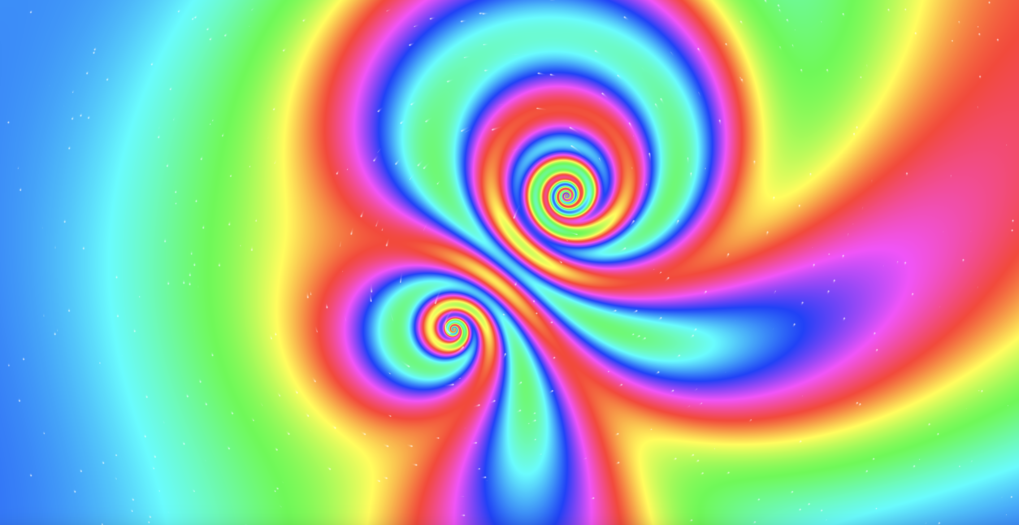
Rainbow

Rainbow is perhaps the most simple algorithm in terms of code complexity, but is able to generate a wide variety of outputs. There are no discontinuities in the flow field rendering, making it look like a subsonic flow field with no shockwaves. Rainbow typically animates slowly and displays a smooth, full spectrum of colors that dance together seamlessly.

Form

Form attempts to more intentionally expose the structure and shape of the modified “streamlines” used by Flows. Hard edges of color in a sea of darkness expose the underlying forms of the flow fields. The blending of colors into darkness were somewhat inspired by aurora borealis, which is controlled by many things, one of which is magnetic field lines, which may also be modeled in ways that satisfy Laplace’s equation (compare potential flow doublet and magnetic dipole).

Step

Step focuses heavily on the rings of color surrounding sources and sinks. The colors slowly animate and change color, but remain blended in a rippled pattern. The ripples in color were partially inspired by oscillations often observed in numerical flow simulations, especially in flow regions with high rates of change, such as a shockwave. Since numerical simulations are typically rendered with a color gradient range limited from red to blue (excluding magentas and purples), this color palette also limits its colors to the same range of colors.

Skip

Skip is also inspired by numerical simulations. Numerical simulations of aerodynamic flows with shockwaves can unintentionally introduce spurious oscillations. Skip takes inspiration from this and winds itself up with oscillatory shapes of color bands. Periodically, the color bands will “skip” over themselves in a discontinuous manner, drawing inspiration from the discontinuous nature of shockwaves. Since numerical simulations are typically rendered with a color gradient range limited from red to blue (excluding magentas and purples), this color palette also limits its colors to the same range of colors.

Monochromatic

Monochromatic attempts to produce compelling outputs that depict the underlying flow field while only using a single hue. Structures and shapes within the flow are exposed through adjustments to saturation and brightness only.

I think Monochromatic has some of the most interesting outputs. By limiting colors to a single hue, some flow features become more clearly defined.

Inclusion

Inclusion is a special palette inspired by my son born with Down syndrome. The outputs are blue and yellow, representing Down syndrome awareness. This palette continues the tradition of Friendship Bracelet’s Inclusion palette that Alexis André graciously let me provide input on.

Only token #321 will have this color palette. The number 321 is commonly used to celebrate Down syndrome because people with Down syndrome have three chromosomes on their twenty-first chromosome.

Selected Testnet Outputs

A few selected Goerli testnet outputs are displayed below as static images.

Note: Flows is best viewed as an animated piece because it attempts to convey fluid motion to the viewer, however, many methods of displaying artwork are limited to static images, and renderings of a single frame sometimes are the only option.

Conclusion

I’ve had a lot of fun exploring within the Flows algorithm. I hope the outputs bring joy to others, and I hope it inspires some to consider learning more about aerodynamics.

---

For additional commentary on flow visualizations and how they relate to generative art, see my blog post, Seeing the wind.